 |
|||||||||||||||
|
|
|||||||||||||||
|
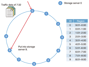
Feature Articles: New Generation Network Platform and Attractive Network Services Vol. 14, No. 3, pp. 33–38, Mar. 2016. https://doi.org/10.53829/ntr201603fa5 Distributed Time Series Data Management and AnalysisAbstractAt NTT Network Innovation Laboratories, we are studying sophisticated network management schemes based on network data analysis. In this article, we focus on a distributed data analysis scheme for large amounts of network data. With this scheme, the amount of network data transported among datacenters for analysis can be reduced, which will also reduce costs. Keywords: distributed database, distributed data analysis, skiplist 1. IntroductionSensor data and traffic data have recently come to be stored in datacenters. Analyzing such data makes it possible to predict traffic jams and network congestion. These data are generated with high frequency, and the amount becomes increasingly larger as time goes on. This means that data cannot be managed in a general relational database because a relational database constructs a rigorous data structure and sacrifices the scalability of data management. A key-value store (KVS)*1 is a simple data storage architecture widely used to manage large amounts of data because it stores only simple key-value pairs (Fig. 1). MapReduce*2 is a well-known distributed data analysis scheme that has good scalability for analyzing large data sets in parallel, and it is easily built and deployed on KVS [1]. If all data are distributed fully into KVS, MapReduce quickly achieves parallel data analysis. The performance of MapReduce can be guaranteed in simple cases of data analysis; however, it is difficult to apply it for complex analysis such as time series data analysis and distributed machine learning. The specific difficulties are as follows.
(1) Currently, the nodes’ states are managed in a centralized server in a general MapReduce platform such as Hadoop [2]. Therefore, the load on the centralized server may exceed capacity as the number of analysis executions increases. (2) The ideal parallel performance of MapReduce is guaranteed in that all data sets are fully distributed in KVS. However, time series data may be non-uniformly distributed in KVS. For example, if a large amount of data is concentrated on certain servers, the performance of MapReduce analysis will be degraded. (3) In machine learning analysis using MapReduce, there is frequent data communication among all nodes (i.e., the shuffle phase), and this causes heavy traffic and network congestion. We have been researching a MapReduce architecture to solve these problems. In this article, we introduce an efficient MapReduce architecture based on distributed skiplist tree (DST) [3].
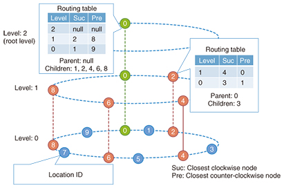
2. MapReduce scheme based on DSTDST is a hybrid data structure consisting of both a balanced tree and a linked list such as a skiplist, which takes only O(log N) operations to search/put/remove data. To construct a DST in a distributed environment, each node has two values: the location identification (ID) and the level. The location ID is the circulated hashed ID, which is used to determine the ID space region of a node. The level refers to the hierarchy level in the DST, which is determined by the function of [-logK RAND], where K and RAND are denoted as the balancing factor and the random value among [0,1], respectively. Using this function to determine the hierarchy level, we obtain the probability (1/K)l of a node being located at level l. All nodes in the hierarchy of the node at level 1 must be placed below level 1, and that node connects all nodes between the node location ID and its neighbor at level l. In this way, all of the connections form a DST (Fig. 2). The DST achieves a balanced tree without balancing operations; therefore, the maintenance cost of a balanced tree is very low.
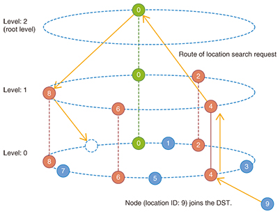
Next, we describe the DST construction procedure consisting of node join/leave operations. When node P (location ID p and level l) joins the DST, it requests an existing node to search its own location in level l. The node receiving the request checks whether location ID p is between its own ID and its neighbor’s ID in level l. When the location ID p is not in the ID region, the receiving node forwards the request to its own parent node. In contrast, when the location ID p is in the ID region, the receiving node forwards the request to the child nodes closest to location ID p. In repeating the request forwarding, the request arrives at the node containing p in its own location ID region. Then, that node divides its own ID region into two ID regions for itself and for node p, and becomes the neighbor of node P. The summarized procedure for a node to join the DST is that a neighbor search operation using O(log N) request forwarding is carried out (Fig. 3).
When a node leaves the DST, the node does not inform the other nodes of its leaving. Therefore, the nodes must monitor each other using a heartbeat*3 protocol in order to handle the situation when nodes leave. The heartbeat protocol involves simple synchronize/acknowledge (SYN/ACK) communications among nodes. The protocol sends a SYN message to a node and checks whether a corresponding ACK reply is received. In DST, each node checks child node states using the heartbeat protocol. If a parent node detects that a child node has left, the parent node searches for the node neighbor and replaces the leaving node. If the parent node recognizes the neighbor node, the leave is fixed by a few network communications. In the worst case, the parent node must search for the neighbor node from the entire DST. However, it takes only O(log N) message forwarding by using the search protocol introduced in the node join procedure. The cost of these node join/leave operations is only O(log N) message forwarding; therefore, DST achieves scalable/distributed node management and solves problem (1) mentioned in section 1. Next, we introduce the load balancing function in DST. A root node located at the highest level periodically requests load information (e.g., the number of receiving queries per hour) from its child nodes, and the receiving nodes forward the requests to their child nodes recursively. When the request arrives at the nodes in level 0, the nodes send information about their own load to the parent node. The parent node sorts the information in descending order of load and forwards the top and bottom A load information to its own parent node. Through recursive execution of this process, the root node obtains the top and bottom A load information from the DST and balances the popular data among the 2A nodes. This process is repeated periodically, and the DST is able to balance the entire load step-by-step, solving problem (2) mentioned in section 1. Finally, we introduce a traffic reduction scheme generated by the MapReduce process in the DST. All data in the MapReduce process are delivered to their destination nodes through the DST. Then, each parent node combines the delivered data destined for the same nodes and redelivers them. The efficiency of this traffic reduction scheme depends on the characteristics of the time series data, but it is expected to achieve a significant reduction in traffic compared with naive delivery and to solve problem (3) mentioned in section 1.
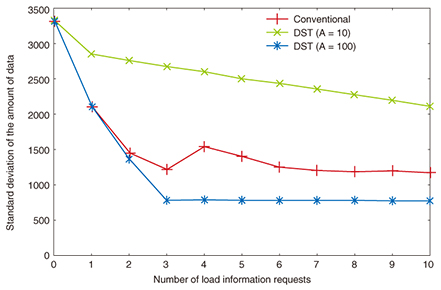
3. EvaluationWe evaluated the performance of DST through computer emulation. In this emulation, there were 1000 nodes, and each node had [0, 10,000] time series data with a time range of [00:00, 23:59]. For comparison, we also evaluated the MapReduce platform based on Microsoft Azure [4]. First, we evaluated the effectiveness of load balancing. In the evaluation, we set variable A as 10 or 100 and measured the standard deviation of the amount of data among nodes while changing the number of load information requests (Fig. 4). We observed from the results that the effectiveness of load balancing in DST was higher as A became larger even if the number of requests was small.
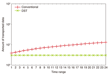
Next, we evaluated the amount of data transported in the MapReduce process when the target time range was changed. The results indicated that DST effectively reduced the amount of transported data as the target range was expanded (Fig. 5).
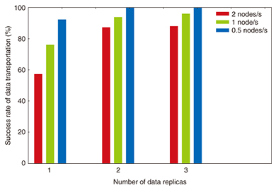
Finally, we evaluated the stability of DST in a churn environment, which is where some nodes frequently join/leave the DST and also replicate data to other nodes more frequently. The frequencies of joining/leaving were set at 0.5, 1, and 2 per second, and each node replicates data it holds in one to three of its closest neighbors. In this environment, each node repeatedly sends certain kinds of data to the other node/s at an interval of 0.2 s. We measured the average success rate of the data transportation (Fig. 6). The results indicated that the success rate is significantly improved as the number of replicas increases.
4. Summary and future workIn this article, we introduced the DST and evaluated its effectiveness through emulation. The next step is to discuss the DST architecture with skiplist experts and work on making it even more effective. In addition, we will verify the effectiveness of DST when it is used to analyze real traffic data. References
|
|||||||||||||||

