Complex Data Analysis Using Mixture Models

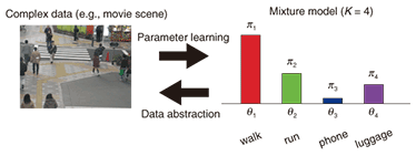
1. Introduction

Nowadays, many people enjoy a vast amount of digital data such as text, images, music, and videos downloaded from the Internet via broadband network access. Surveillance cameras automatically capture public scenes every day, and these videos are stored in huge data repositories. In stock markets, automated computer agents generate a huge amount of transaction records for every second.

Since the available datasets are so huge that no human can analyze them manually, many researchers have tried to use statistical and probabilistic models to analyze their complex properties. Typically, these models represent complex data by a stochastic process (model) with a few parameters. These parameters are tuned (trained) by machine learning [1] techniques to explain the observed data as much as possible: the idea is that if we can explain the observation set well, we may have some confidence that the learned parameters and the chosen model represent (part of) the essence of the data.

Many statistical models have been proposed for complex data analysis. One of the most popular techniques uses mixture models, which have proven to be very useful in many studies and domains. A mixture model assumes that the observed data are generated by a small number of hidden components, each of which has different parameters (characteristics). The model estimates the properties of this mixture of hidden components from the given data.

This article explains the idea and the usefulness of mixture models and their extension for complex data analysis. It also introduces an application of the mixture model to the field of computer vision for target tracking. Section 2 explains a standard mixture model using an example of movie scene understanding. Section 3 introduces a recent mixture model extension. Section 4 reports research by my colleagues and I on target tracking and shows some results.

2. Mixture model

Assume that we have a camera that captures an ordinary scene of pedestrians on a street in Tokyo. Many people are visible in the scene. The captured images include many human activities: some people are just walking, but their walking directions and speeds are different; a few business people walk rapidly while using cell phones; and some kids are running around. How can we model, or represent, such complex information with a statistical model?

The mixture model assumes that these complex data are generated by a number of different sources. Each source is called a component, characterized by a unique pattern of data outputs. We understand the given data as the mixture of these different patterns generated from the multiple components. In this example, people are generating the visual stimuli. We assume that personal behavior can be categorized into a manageable number of patterns: walking, running, using cell phones, carrying luggage, etc. A complex scene with a number of people can be decomposed into several behavior patterns. That is, a captured video can be understood as a (complex) mixture of these different sources (Fig. 1).

Fig. 1. Illustration of mixture model.

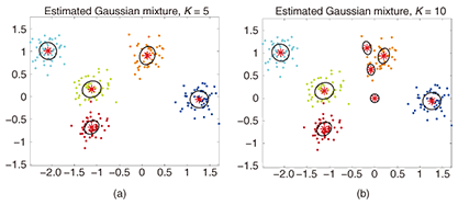
More technically, the mixture model assumes that K hidden (latent) components with different parameters (characteristics) θ_k underlie the observed data X = {x_i}. Each portion of the observed data is generated from one of these hidden components, and the total amount of data generated by component k is defined by its mixing ratio π_k. The model is formulated as follows:

where p(x) denotes the probabilistic density function of predicate x and

We tune (learn) the parameters θ_k and the mixing ratios π_k of these hidden components in order to approximate the given observed data. This parameter learning can be carried out automatically by maximizing a standard evaluation function.

Some results of using a mixture model to analyze a set of two-dimensional (2D) points are shown in Fig. 2. The small colored dots denote data points. The dataset is assumed to be generated by five mixture components. Each point is generated from one of the five components where its color indicates the source component. Each component is modeled as a 2D Gaussian distribution and generates 50 data points. Red stars and corresponding black ellipses indicate the means and standard deviations of estimated Gaussian components yielded by the Gaussian mixture model. K is fixed and the model is fitted using the variational Bayes method [1], which is an iterative computation technique. Figure 2(a) is the result when the correct value of K = 5 was chosen, while Fig. 2(b) shows an example of an incorrect value, K = 10. As shown, the mixture model can derive reasonable mixture component distributions if the specified K is correct.

Fig. 2. Mixture model results estimated from 2D data points with (a) the correct K = 5 and (b) an incorrect K = 10. Three components overlap at (0, 0) in (b).

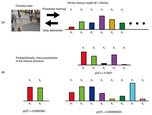
Mixture models are basic yet practical tools in many problems in several domains. For example, a mixture model can be used to describe the background scenes of a movie [2]; the key advance is distinguishing the foreground objects that are the focus of attention from the background. Since the background has many different surfaces and planes, its pixel values can be effectively modeled by a mixture of different pixel value components. A mixture model has also been used for automatic speaker recognition in recorded sounds [3].

3. Infinite mixtures obtained by nonparametric Bayes models

One problem with using mixture models is that we have to determine K in advance. In general, specifying the correct K is very difficult, and using the wrong value of K may degrade model fitting very badly, as seen in the example (Fig. 2(b)). One popular solution is to use an information criterion for choosing the best K, i.e., AIC [4] or BIC [5]. In this case, we prepare several mixture models with different K values and compute the criteria for each learned model.

Recently, another solution, called the nonparametric Bayes approach, has been developed. It does not demand that K be specified. Instead, the model chooses an appropriate value for K to explain the given data in a probabilistic manner.

In this article, I introduce the Dirichlet Process Mixture (DPM) model, a nonparametric Bayes extension of usual mixture models. Mathematically, DPM represents a mixture of infinitely many components (Fig. 3(a)). Thus, it has the potential to fit any mixture. It assumes many possible mixture structures G¹, G², …, probabilistically (Fig. 3(b)). Some mixtures have higher probabilities and others have lower probabilities. In practice, we have only a finite amount of data information: i.e., the number of components cannot be infinite. DPM chooses the most appropriate mixture structure––the values of K and π_k––from infinitely many candidates.

Fig. 3. Illustration of DPM model.

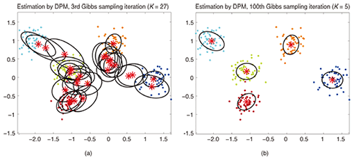
A more mathematically precise explanation is given below. Formally, DPM is based on the Dirichlet process, which is a stochastic distribution of distributions. However, explaining how DPM can be based on a Dirichlet process is not intuitive in the context of the mixture model. Therefore, I explain DPM from the mixture model viewpoint. The resulting probabil-istic distribution of parameters θ is described as follows:

There are two points to note. First, index k imposes no upper limit on K in the summation in Eq. (2). This indicates that DPM is an infinite mixture model. Second, Stick(γ) is a stochastic process called the stick breaking process [6]. The stick breaking process (Eq. (3)) randomly generates an infinite number of positive scalars that are summed to one. More precisely, Stick(γ) generates πk according to the following equations:

This indicates that the structure of the mixture, including the number of components and their mixing ratios, is defined in a stochastic manner rather than a deterministic manner: that is, it is defined on the basis of sampling from the Beta distribution. Note that π_k rapidly decreases as k becomes large because of the product of v_k. Therefore, the stick breaking process inherently offers a clustering function: the process does not want the mixing ratios to be large for many of the components. Given G(θ), the observed data X = {x_i} is modeled in the same way as the original mixture models, except for an infinite number of components:

One reason for using DPM is that the number of clusters automatically scales with the data complexity, and we can automatically find a mixture with an appropriate number of components using a standard Bayes (probabilistic) machine learning technique. As noted, by using DPM we can avoid the need to specify the number of mixture components, a key weakness of mixture models.

Another advantage of DPM is that it provides an easy and convenient formulation. Implementing the above infinite equations (Eqs. (2) and (3)) in a program (with finite memory) is difficult. One solution is the Chinese restaurant process (CRP) [7]. In CRP, each observed datum (point) is assigned to one of the mixture components. Let us denote the assignment of the ith item x_i to the kth component as z_i = k. Moreover, let us denote the total number of data as N. In CRP, we use the following rules to determine z_i:

This equation computes the probability of the ith datum being assigned to the kth component under the condition that the assignments of all other data are fixed. Here, n_k denotes the number of items assigned to the kth component and K denotes the number of components, counted via N-1 assignments. CRP assigns the ith datum to the kth component with a probability proportional to the component’s membership. The probability of a new K+1th cluster being generated is proportional to γ.

We repeat this process many times with different values of i and achieve assignments for all data. During the process, the number of mixture components varies. It is known that CRP-based DPM is truly equivalent to the formal infinite representations of Eqs. (2) and (3).

A simulation result for DPM is presented in Fig. 4. We tested the same dataset as used in Fig. 2 and estimated the hidden mixture structure by using DPM. We used a CRP representation of DPM and chose Gibbs sampling [1] as the inference algorithm. Figure 4(a) shows a result in an early iterative step and Fig. 4(b) is the final result indicated by the convergence of the Gibbs computation. As can be seen, DPM obtained the correct K = 5 mixture components. Let me emphasize again that there was no need to specify the initial value of K: the model automatically found the best K to represent the given data.

Fig. 4. Mixture model results estimated from 2D data points by using DPM. (a) An early result (third iteration). The inference has not converged yet, and the estimation is not good. (b) After convergence of the Gibbs sampling, the correct mixture structure with K = 5 components was recovered automatically.

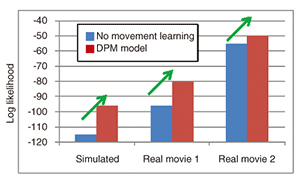
Because of this advantage, many researchers have applied DPM to many problems, including community detection from network data [8] and document (natural language) modeling [9].

4. Application: multi-target tracking with movement pattern discovery

Here, I describe our work on using the mixture model to understand visual scenes. Many developed countries and major cities have visual surveillance cameras for security. These cameras are useful for deterring crimes and the captured data can be used to identify accidents or criminal activities. However, it is said that surveillance cameras, by themselves, are not so effective in deterring truly committed criminals or terrorists. Detecting anomalous activities as precursors to illegal acts still requires human eyes and it is impossible for all cameras to be adequately covered by human observers.

To enable automatic analysis of video streams, many researchers have studied the problem of action recognition and scene understanding; for example, identifying suspicious activities. The technique of tracking, which is one of the hot research topics in this field, is intended to locate and follow particular people against various backgrounds. More technically, tracking should determine the parameters of the objects of focus such as their locations and postures. The most common security concern is to track humans (in many cases, pedestrians), and many studies have, of course, addressed this task (e.g., [10]–[15]).

The outputs of surveillance cameras contain many patterns or target movements: the targets run, walk, and turn at various speeds and in various directions, and objects change their movement to avoid collisions and follow signals. However, many tracking models assume that the movement patterns of the targets (pedestrians) are invariant. Detecting such changes in movement patterns will yield more precise tracking. One problem is that we do not know the exact, or best, number of such movement patterns. Moreover, it is clear that these patterns are context-dependent: different patterns are exhibited at airports, train stations, and shopping malls and on the street.

We have developed a tracking algorithm that can solve these problems by using the DPM model [16]. Using DPM, we can automatically obtain an appropriate number of movement patterns that fit the scene’s context. Our developed model can also learn these patterns in an online manner: in other words, it discovers a novel pattern appearing in a video at first sight.

We tested our model with three datasets: one simulated and two real video sequences. A quantitative result using log likelihood as a data fitness measure is shown in Fig. 5. Our model outperformed a conventional model, which was unable to discover movement patterns.

Fig. 5. Log likelihood comparison results. Larger log likelihoods are better.

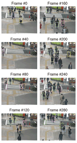
A tracking result for an actual video sequence is shown in Fig. 6. Colored rectangles indicate the tracked targets, and the number above the rectangle is the movement pattern index for that frame. As you can see, a target can exhibit different movement patterns over time.

Fig. 6. Tracking results obtained by DPM.

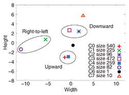
The discovered movement patterns θ_k for the same dataset are shown in Fig. 7. We found six major movement patterns. Upward and downward movements had two subpatterns, corresponding to leftward or rightward movements. Right-to-left movements exhibited a slow movement pattern (green cross) while a fast movement pattern had fewer instances (purple circle). This differentiation well matches the actual sequence: a few persons walked rapidly, but the majority walked slowly. Note that these movement patterns were automatically discovered by the infinite mixture model based on DPM.

Fig. 7. Movement patterns discovered by DPM. Size indicates how many times pattern Ci occurred in the movie.

5. Conclusions

In this article, I introduced mixture models for analyzing complex data such as video sequences. A standard mixture model, used in many applications, uses a fixed number of mixture components K. DPM is a recent development that assumes (mathematically) an infinite number of mixture components and can therefore adapt to unknown mixtures. My colleagues and I have applied DPM to the target tracking problem. Our system automatically learns movement patterns, and tests showed that it achieved better tracking precision than the conventional solution.

References

[1]	C. M. Bishop, “Pattern Recognition and Machine Learning,” Springer-Verlag New York, 2006.
[2]	C. Stauffer and W.E.L. Grimson, “Adaptive Background Mixture Models for Real-time Tracking,” Proc. of the IEEE Computer Society Conference on Computer Vision and Pattern Recognition (CVPR), Ft. Collins, USA, 1999.
[3]	D. A. Reynolds, T. F. Quatieri, and R. B. Dunn, “Speaker Verification Using Adapted Gaussian Mixture Models,” Digital Signal Processing, Vol. 10, No. 1–3, pp. 19–41, 2000.
[4]	H. Akaike, “A New Look at the Statistical Model Identification,” IEEE Trans. Automatic Control, Vol. 19, No. 6, pp. 716–723, 1974.
[5]	G. Schwarz, “Estimating the Dimension of a Model,” Annals of Statistics, Vol. 6, No. 2, pp. 461–464, 1978.
[6]	J. Sethuraman, “A Constructive Definition of Dirichlet Process,” Statistica Sinica, Vol. 4, pp. 639–650, 1994.
[7]	D. Blackwell and J. B. MacQueen, “Ferguson Distributions via Polya Urn Schemes,” The Annals of Statistics, Vol. 1, No. 2, pp. 353–355, 1973.
[8]	C. Kemp, J. B. Tenenbaum, T. L. Griffiths, T. Yamada, and N. Ueda, “Learning Systems of Concepts with an Infinite Relational Model,” Proc. of the 21st National Conference on Artificial Intelligence (AAAI), pp. 381–388, Boston, USA, 2006.
[9]	D. Mochihashi, T. Yamada, and N. Ueda, “Bayesian Unsupervised Word Segmentation with Nested Pitman-0yor Language Modeling,” Proc. of the Joint Conference of the 47th Annual Meeting of the ACL and the 4th International Joint Conference on Natural Language Processing of the AFNLP (ACL-IJCNLP), pp. 100–108, Suntec, Singapore, 2009.
[10]	M. Andriluka, S. Roth, and B. Schiele, “People-tracking-by-detection and People-detection-by-tracking,” Proc. of IEEE Computer Society Conference on Computer Vision and Pattern Recognition (CVPR), Anchorage, USA, 2008.
[11]	N. Dalal and B. Triggs, “Histograms of Oriented Gradients for Human Detection,” Proc. of IEEE Computer Society Conference on Computer Vision and Pattern Recognition (CVPR), Vol. 1, pp. 886–893, San Diego, USA, 2005.
[12]	H. Grabner and H. Bischof, “On-line Boosting and Vision,” Proc. of IEEE Computer Society Conference on Computer Vision and Pattern Recognition (CVPR), Vol. 1, pp. 260–267, New York, USA, 2006.
[13]	Z. Li, Y. Li, and R. Nevatia, “Global Data Association for Multi-object Tracking Using Network Flows,” Proc. of IEEE Computer Society Conference on Computer Vision and Pattern Recognition (CVPR), Anchorage, USA, 2008.
[14]	B. Leibe, N. Cornelis, K. Cornelis, and L. Van Gool, “Dynamic 3D Scene Analysis from a Moving Vehicle,” Proc. of IEEE Computer Society Conference on Computer Vision and Pattern Recognition (CVPR), Minneapolis, USA, 2007.
[15]	B. Leibe, K. Schindler, N. Cornelis, and L. Van Gool, “Coupled Detection and Tracking from Static Cameras and Moving Vehicles,” IEEE Trans. on Pattern Analysis and Machine Intelligence, Vol. 30, No. 10, pp. 1683–1698, 2008.
[16]	K. Ishiguro, T. Yamada, and N. Ueda, “Simultaneous Clustering and Tracking Unknown Number of Objects,” Proc. of IEEE Computer Society Conference on Computer Vision and Pattern Recognition (CVPR), Anchorage, USA, 2008.

↑ TOP