How Number Theory Elucidates the Mysteries of Complex Dynamics—Viewed through
Non-Archimedean Dynamics

1. Introduction

The theory of complex dynamics is a field in mathematics that studies asymptotic behaviors of dynamical systems defined from recurrence formulae with complex coefficients. For instance, the formula , parametrized by a complex number c, represents the dynamics over the complex plane. That is, if we set an initial state x₀, which is a complex number, the states x₁, x₂, x₃, … are determined sequentially with the formula. The question is what happens to x_n when we consider n → ∞. Despite the simple form of the formula, the answer is deeply related to rich and intriguing structures such as the Mandelbrot set (Fig. 1).

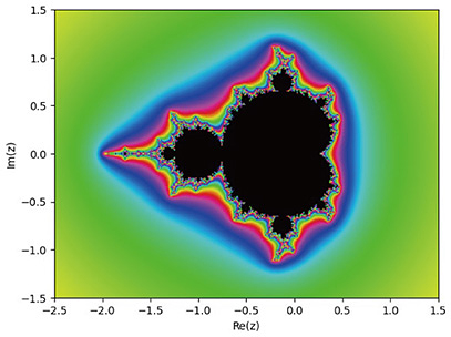
Fig. 1. The Mandelbrot set.

Research in this field is fascinating because of its crucial connections with other areas, such as real dynamics, arithmetic dynamics, non-archimedean dynamics, algebraic geometry, and Arakelov geometry. These areas have their methods and purposes but affect each other, i.e., if one field has significant progress, it stimulates and is applied to different fields. In this article, we explore this connection from the example of a relation between complex dynamics and non-archimedean dynamics, which is the author’s field of study, after we look at what precisely complex dynamics involves.

2. Complex dynamical systems

Let us consider the example that appeared in the previous section. The simplest case is when c = 0, that is, . Since the recurrence formula has a solution x_n = (x₀)²ⁿ, we can see the asymptotic behavior depending on the absolute value of the initial state x₀ as follows:

(a)   Case |x₀| < 1: {x_n} converges to 0;

(b)   Case |x₀| > 1: {x_n} diverges to ∞;

(c)   Case |x₀| = 1: |x_n| stays 1 for any n.

In cases (a) and (c), the asymptotic behaviors are stable under small fluctuation of x₀ while it is not in case (b). That is, in case (a) (resp. (c)), if we give a slight change to x₀ so that |x₀| < 1 (resp. |x₀| > 1) still holds, the asymptotic behavior, converging to 0 (resp. diverging to ∞), does not change. In case (b), however, small fluctuation of an initial state affects its asymptotic behavior; if the absolute value |x₀| becomes smaller (resp. greater) than 1, case (b) becomes (a) (resp. (c)). The set of unstable points under slight fluctuation is called the Julia set. In this specific case of the dynamical system defined by , the Julia set is the set of point x₀ with |x₀| = 1, namely the unit circle in the complex plane ℂ. It has a simple shape, a circle as in Fig. 2, but this is special. For instance, Fig. 3 shows the Julia set of the dynamics with c = –1. This set is called “Basilica” because of its shape. Fig. 4 is the Julia set “Rabbit” of the dynamics with c = 0.123 + 0.745i, and Fig. 5 is “Airplane” that appears when c = –1.75488. We see how myriad shapes of the Julia set appear by simply taking various c’s in the formula .

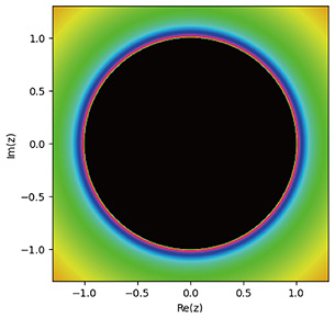
Fig. 2. The Julia set at c = 0.

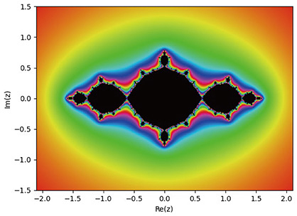
Fig. 3. The Julia set at c = –1, “Basilica.”

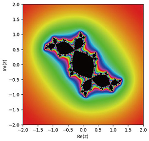
Fig. 4. The Julia set at c = –0.123 + 0.745i, “Rabbit.”

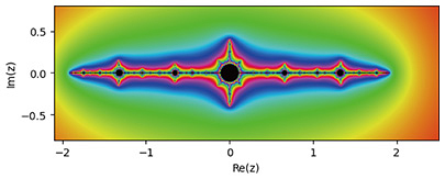
Fig. 5. The Julia set at c = –1.75488, “Airplane.”

The Mandelbrot set controls the shape of Julia sets attached to the dynamics . Let us take a look at it more closely. It is a subset of the parameter space of , i.e., the space of c, which has a complicated shape with many areas divided by it. The meaning of this set is as follows. Each time you take point c from the complex plane, where the Mandelbrot set lives, it corresponds to a recurrence formula , the dynamics defined from it, and the Julia set of it. If one moves c continuously, it is reasonable to expect that the Julia set moves continuously along the motion of c. Intriguingly, it was found that this was different and the true description was as follows. The motion is continuous only if one takes the parameters inside an area divided by the Mandelbrot set. In this case, the Julia sets’ shapes look similar. However, once one crosses the border, it is no longer the case. For example, c = 0 lies inside the area that looks like a cardioid (the widest area), c = –1 inside the area to the left of the cardioid that looks like a disk, and c = 0.123 + 0.745i inside the area above the cardioid that looks like a disk, which means they lie in areas different to each other. The Julia sets keep their shape inside each area. However, the shape changes completely when the area moves from one area to another. The motion of the Julia set is unstable under small fluctuations on the boundary of the Mandelbrot set. Such a phenomenon, the drastic change in shapes of the Julia sets with slight fluctuation of parameters, is called bifurcation, and a parameter at which the bifurcation occurs is called a bifurcation point. The Mandelbrot set is the set of bifurcation points of c in the recurrence formula . The Julia set controls the stability of asymptotic behaviors for fixed c while the set of bifurcation points (or the Mandelbrot set in this specific example) controls the stability of motion of the Julia sets when we fluctuate the dynamical systems along parameters.

The Julia sets and Mandelbrot set have quite rich and interesting properties. As shown in Figs. 2–5, the various Julia sets look complicated but have rules inside the structure, called self-similarity. The Mandelbrot set has a similar property. If one zooms in on part of it, another Mandelbrot-look-alike set appears inside the Mandelbrot set, as in Fig. 6. It is fascinating, but at the same time, quite difficult. A case in point is the property of the so-called local connectivity of the Mandelbrot set, which is still open.

We can define similar stabilities, i.e., the notion of Julia sets and the sets of bifurcation points for different recurrence formulae. For instance, when we consider a polynomial ƒ of more than two degrees in the formula x_n+1 = ƒ(x_n), its parameter space can be higher dimensional. We can also consider dynamical systems with higher dimensional phase spaces. An Hénon map defines a crucial example of such dynamics that has been studied actively. It is represented by the recurrence formula , x_n), where a and b are complex numbers with b ≠ 0. Hénon devised it as real dynamics, i.e., x_n, y_n, a, b are all real numbers, to initially study the chaos phenomena generated from a differential equation called the Lorentz equation that simulates climate. Mathematicians later observed interesting phenomena unique to complex versions of the dynamics of the Hénon maps, and even several applications to real Hénon maps. This is a part of an interaction between real and complex dynamics.

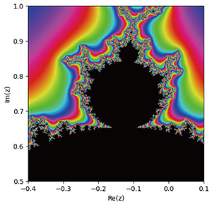
Fig. 6. The Mandelbrot set zoomed at [–0.4, 0.1] × [0.5, 1.0].

3. Non-archimedean numbers and non-archimedean dynamics

Just as complex dynamics is a theory of dynamical systems over complex numbers, non-archimedean dynamics treats dynamical systems over non-archimedean numbers. Non-archimedean numbers is a name for several types of numbers with a common property called non-archimedes. The most typical example of a non-archimedean number is the p-adic number, which we take as an example to see what non-archimedes is. The “p” inside the p-adic number is a prime. There are 2-, 3-, 5-adic numbers, …, and they are lateral to complex and real numbers. Another typical example is called the Laurent series, which we discuss later. Let us look at the properties of non-archimedean numbers from an instance of 2-adic numbers.

Consider a metric on the set of integers, which is different from the usual one and called 2-adic distance, given by the following rule. The more times the difference of two numbers is divisible by 2, the closer they are to each other. We observe this rule by an example. In a usual metric, 4 is closer to 2 and further to 8. However, the difference between 2 and 4 is 2, which is divisible by 2 once, while that between 4 and 8 is 4, which is divisible by 2 twice. We conclude that 8 is closer to 4 than 2 with respect to the 2-adic metric.

The 2-adic distance is deeply related to the 2-adic expansion, i.e., the binary representation of numbers. The 2-adic expansions of the above three numbers are

2 = (10)₂;

4 = (100)₂;

8 = (1000)₂.

When we compare their distance, we need to read the 2-adic expansions from right to left. We observe that the first two digits coincide in the 2-adic expansions of 4 and 8, while only one digit is in those of 2 and 4. Comparing the above rule of the 2-adic distance with the definition of the 2-adic expansion, we see an alternative, but the equivalent rule of the 2-adic distance is the more digits of the 2-adic expansions of two numbers coincide, the closer they are to each other when we read the expansion from right to left. More precisely, it is conventional that the distance of two numbers, the 2-adic expansion of which shares the same first n digits, is defined as 2^–n. We write the 2-adic distance of two positive integers a and b as d₂(a, b).

Let us now extend the metric. We consider a 2-adic expansion (⋯111)₂ that continues infinitely to the left. By definition, it is the limit of the sequence (1)₂, (11)₂, (111)₂, …, i.e., 1, 3, 7, …. They look to diverge to infinity but converge to –1 in the 2-adic distance. By adding 1 to this sequence, we obtain a sequence (10)₂, (100)₂, (1000)₂, …, which converges to 0. More specifically, the 2-adic distance between (10)₂ = 2 and 0 is 1/2, that between (100)₂ = 4 and 0 is 1/4, and that between (1000)₂ = 8 and 0 is 1/8, …. We see that the distance converges to 0, i.e., (⋯111)₂ + 1 = 0, which means (⋯111)₂ = –1. The 2-adic distance can naturally extend to numbers written as a 2-adic expansion that continues infinitely to the left, such as (⋯111)₂ = –1 above.

We can consider decimals as we do in real numbers. In the 2-adic expansion, there are halves place, quarters place, 1/8 place, etc. It is natural, by the exponential law, to regard these as being divisible “1 times,” “–2 times,” and “–3 times,” respectively, by 2. Namely, we have d₂(1/2, 0) = 2, d₂(1/4, 0) = 4, d₂(1/8, 0) = 8, …. and clearly this sequence diverges to ∞. Recall that in a standard distance, a sequence, where the number of digits to the left of the decimal point increases, diverges, while a sequence, where the number of digits after the decimal point increases, does not. The opposite is true for the 2-adic distance.

Now let us define the 2-adic numbers. The 2-adic numbers are the 2-adic expansions with an infinite digit to the left of the decimal point and finite digit to the right. Note that a number with infinite digits to the left of the decimal point can be obtained as the limit of the finite-digit numbers obtained by truncating the n-th digit. The sequence of these truncated numbers converges by the above argument. We extend the 2-adic distance considered above to the set of 2-adic numbers, and it is possible to assess convergence and divergence. With a few arguments, we can show that the set of 2-adic numbers contains all the rational numbers, including the positive integers we considered first and the negative integers such as –1 = (⋯111)₂. In this sense, we can say that the set of 2-adic numbers is similar to that of real numbers: they both have distances and limits (so-called “completeness”) and include all the rational numbers. However, we can also say they differ from other perspectives, most of which come from the property of the 2-adic distance, i.e., non-archimedes. The 2-adic numbers are non-archimedean, which means the strong triangle inequality holds. For any 2-adic numbers a, b, and c, we have d₂(a + b, c) ≤ max(d₂(a, c), d₂(b, c)). Because 2 is divisible by 2 once and 4 twice, 2 + 4 is divisible once, which is the minimum number of times that they are divisible by 2. Since this “1” in “once” appears in the 2-adic distance of 2 and 4 d₂(2, 4) = 2^–1, with –1 multiplied, the “minimum” appears as maximum in the inequality of distance. By putting any positive real numbers in a, b, and c, this inequality does not hold for the usual distance of real and complex numbers (remark: the triangle inequality d(a + b, c) ≤ d(a, c) + d(b, c), the weaker form of the strong triangle inequality holds instead). That is, the strong triangle inequality is unique to 2-adic numbers. Let us next discuss the difference the strong triangle inequality makes between real and 2-adic numbers.

Let us look at the difference in “shapes” of the sets of real and 2-adic numbers. Real numbers can be seen as points on a number line, which means the shape of the real numbers is a line. The question is, what is the shape of 2-adic numbers? We derive the answer from the 2-adic expansion. Consider the 2-adic numbers without decimals and describe their 2-adic expansion as a binary tree. This tree starts from one root, with two edges extending, each corresponding to the first digit (counted from the right) 0 and 1. In the same manner, from each node at the end of the edges, two more branches extend, corresponding to the second digit of the 2-adic expansion. Since 2-adic numbers have 2-adic expansion with an infinite digit to the left, we repeat this procedure infinite times. Note that if the number has only a finite digit, we take 0 infinite times. We obtain a rooted tree (Figs. 7 and 8) with infinite depth from this operation. The 2-adic numbers without decimals can then be seen as the set of “endpoints” that is not the first root of this tree. We also acquire the tree for all 2-adic numbers, possibly with decimals, by adding another tree above this tree. We create another rooted tree containing the original one by adding another root corresponding to the halves place, from which two edges extend, and each node at the end of the edge corresponds to one place from each of which the original tree appears. We continue this infinite times to obtain the tree of whole 2-adic numbers, which no longer has a root. The shape of 2-adic numbers is then the set of endpoints of this tree. Not only does each endpoint correspond to a 2-adic number but the tree structure also reflects the distance. As mentioned above, with respect to the 2-adic distance, the more digits of two 2-adic numbers coincide, the closer they are. By tree representation, it is equivalent to saying that the deeper they share edges in the tree, the closer they are.

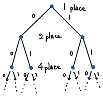
Fig. 7. Binary tree representation of 2-adic expansion.

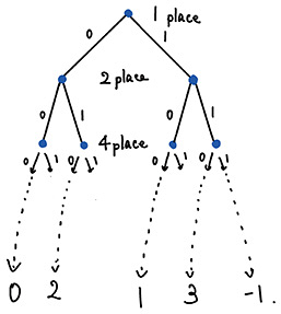
Fig. 8. Binary tree representation of 2-adic expansion with endpoints.

We also see a difference between complex (or real) and 2-adic numbers if we consider the dynamics over them. We have already observed the dynamical system over the complex numbers above. Now, let us look at the same dynamical system, with both phase and parameter spaces 2-adic; x₀ and c are both 2-adic numbers. Because of the limited space, we only consider the formula with c = 0, i.e., . We see that even such a simple dynamical system is good enough to observe the difference. It has a solution , and we can see the asymptotic behavior depending on the absolute value of the initial state |x₀| (that is, defined by d₂(x₀, 0)), (a)–(c) in Section 1, which is the same as the complex case. However, the strong triangle inequality makes the behavior completely different; case (b) is no longer unstable under slight fluctuation of x₀. Let us discuss this in more detail. We take any number ε such that |ε| < 1 and consider x₀ + ε. In the complex case, we saw that the asymptotic behavior was unstable under small fluctuation; for instance, if we take x₀ = 1, then any ε > 0 makes |x₀ + ε| > 1, which is case (a). In the 2-adic case, however, the conditions |x₀| = 1 and |ε| < 1 with the strong triangle inequality indicate that d₂(x₀ + ε, 0) ≤ max(d₂(x₀, 0), d₂(ε, 0)), i.e., |x₀ + ε| ≤ max(|x₀|, |ε|) = 1. Case (a) can never occur with small fluctuation. The condition |ε| < |x₀| also indicates |x₀ + ε| = |x₀|, which is deduced simply by the strong triangle inequality, though we do not present its proof. This means that case (c) cannot occur, either. As a consequence, small fluctuation in the sense of the 2-adic distance does not break the condition in case (b). The dynamics over the 2-adic numbers does not have a Julia set, which is known to be impossible in complex dynamics. We can see how much the non-archimedean property affects the behavior of dynamical systems.

We go back to the first paragraph of this section from the specific number, the 2-adic one. By replacing 2 in the 2-adic distance with other prime numbers, such as 3, 5, and 7, we obtain 3-, 5-, and 7-adic numbers, with the 3-, 5-, and 7-adic distances, respectively. As mentioned above, the p-adic number is a collective term for numbers defined for each prime number. Each set of p-adic numbers has the p-adic distance for which the strong triangle inequality holds as 2-adic distance. Note that they are different from each other; that is, the sets of 2-adic and 3-adic numbers have several common properties, but not the same sets. The p-adic numbers exist as much as the number of the prime numbers, which are infinitely many. As mentioned above, the strong triangle inequality affects the nature of the numbers such as the theory of dynamical systems. Non-archimedean numbers are numbers with a distance that satisfies the strong triangle inequality, which clearly includes p-adic numbers. Even though the examples of the difference between real numbers and non-archimedean numbers (2-adic numbers there) mentioned above may seem peculiar and unintuitive, the p-adic numbers are one of the most fundamental tools in modern number theory, the area of mathematics studying the properties of integers and rational numbers. For instance, p-adic numbers are necessary to prove Fermat’s Last Theorem. In the next section, we examine another application of non-archimedean numbers that are not p-adic.

4. Non-archimedean dynamics and hybrid dynamics

The last topic in this article is devoted to the theory of hybrid dynamics—the application of non-archimedean dynamics to complex dynamics. We take an example as a recurrence formula parametrized by a complex number t. This recurrence formula is unique compared with the above example because we have x_n = 0 for any n when t = 0. We observe that a drastic change, called degeneration, occurs at t = 0, which is not the above-mentioned bifurcation. Bifurcation is a change in asymptotic behavior, not a form of formulae, as in degeneration. Degeneration is related to significant problems associated with the so-called compactification of the moduli spaces. Hybrid dynamics is a strong tool for studying degeneration by means of non-archimedean dynamics. As complex (resp. non-archimedean) dynamics involves the study of dynamical systems over complex (resp. non-archimedean) spaces, hybrid dynamics involves the study of dynamical systems over “hybrid” spaces. The hybrid space was introduced by Boucksom et al. [1] to investigate degeneration phenomena in algebraic geometry. Favre later imported it to study degeneration phenomena in complex dynamics [2].

The non-archimedean number considered in this theory is not a p-adic one but one that is called a complex Lauren series. A (one-dimensional) complex Laurent series is a series , an infinite sum of c_ntⁿ with variable t and complex coefficients c_n, permitting a finite number of negative powers. By complex analysis, every meromorphic function defined around the origin can be written as an infinite sum of such series, i.e., it is an example of the complex Laurent series. Because we do not require any condition on convergence, the Laurent series includes more than just meromorphic functions around the origin. Recalling that a 2-adic number has a binary representation, an infinite sum of 2ⁿ permitting a finite number of negative powers, we can see a similarity between 2-adic numbers and complex Laurent series. It is possible to introduce a distance to the set of complex Laurent series similar to the 2-adic one. If we define that the distance between two complex Laurent series holds for any n ≤ n₀, then the set of the complex Lauren series is a kind of non-archimedean numbers by this distance. Looking at the above example again, the coefficient t = 0 ⋅ 1 + 1 ⋅ t + 0 ⋅ t² + ⋯ is a complex Lauren series. With t regarded as a non-archimedean number, we may consider the recurrence formula as a dynamical system over the set of Lauren series, i.e., non-archimedean dynamics. In other words, we may consider the dynamics of formulas themselves. In general terms, hybrid dynamics describes the relation between the original complex dynamics and induced non-archimedean dynamics.

I drew a rough diagram of the hybrid space in Fig. 9. It is a family of spaces parametrized by a complex number t. Any non-zero t gives just a complex plane, while t = 0 gives the space of the complex Laurent series. The space of the complex Laurent series is the so-called Berkovich space, the details of which are too technical to explain in this short article. Roughly speaking, by considering the Berkovich space, we take into account the whole tree in Fig. 8, not just the set of endpoints where the actual complex Laurent series lives. It is sufficient to have the image in which as the endpoints of the tree structure move according to a recurrence relation, the internal points of the tree also move accordingly. This rough diagram of the hybrid space enables us to regard spaces of non-archimedean numbers as the degenerating “limit” of a family of complex planes, or if it converts into the language of dynamics, hybrid dynamics enables us to regard non-archimedean dynamics as the degenerating “limit” of complex dynamics.

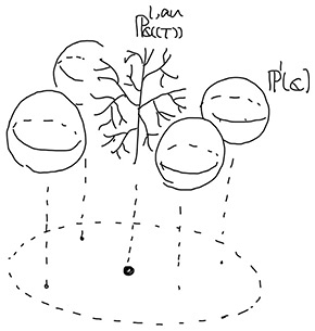
Fig. 9. A hybrid space.

There are several reasons we need such a complicated space. One reason comes from the natural way mathematicians look at mathematical phenomena. As mentioned above, the formula degenerates to a constant when t = 0. Mathematicians consider this phenomenon a wrong consequence by looking at it in an inadequate space. The next question we need to consider is what the “correct” space is to glean a proper degeneration feature. The hybrid space is one possible answer, where the degeneration limit still defines a non-trivial (or non-constant in this case) dynamics.

Favre showed that, for a family of complex dynamical systems whose recurrence formulae are one-variable with one-dimensional parameter t and possibly degenerating at t = 0, the family of Julia sets determined for each non-zero t “converges” to the Julia sets of the induced non-archimedean dynamics, which is a dynamical system over the space of complex Laurent series when we consider everything over the hybrid space [2]. The author presented a similar result for the dynamics of Hénon maps [3], and it is natural to expect to observe similar results in various degenerating complex dynamical systems. Even though non-archimedean numbers may seem odd at first glance, they are essential not only in number theory, as mentioned above, but also in complex dynamics, where non-archimedean dynamics uniformly describe the degeneration of complex dynamical systems.

5. Conclusion

The term “complex dynamics” does not indicate a study method but an area to be studied. Numerous mathematicians study the mysteries in complex dynamical systems with various tools from miscellaneous viewpoints. I gave an example of non-archimedean dynamics. However, mathematicians are constantly presenting more results from multiple approaches every day. I would be delighted if I could share even a glimpse of its importance and allure.

References

[1]	S. Boucksom and M. Jonsson, “Tropical and Non-Archimedean Limits of Degenerating Families of Volume Forms,” Journal de l’École Polytechnique—Mathématiques, Vol. 4, pp. 87–139, 2017. https://doi.org/10.5802/jep.39
[2]	C. Favre, “Degeneration of Endomorphisms of the Complex Projective Space in the Hybrid Space,” Journal of the Institute of Mathematics of Jussieu, Vol. 19, No. 4, pp. 1141–1183, 2020. https://doi.org/10.1017/S147474801800035X
[3]	R. Irokawa, “Hybrid Dynamics of Hénon Mappings,” arXiv preprint: 2212.10851.