Motives—Abstract Art of Numbers, Shapes, and Categories

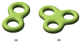
1. What is motive?

In mathematics, it is often the case that two different phenomena/objects show a surprising relationship. Behind such a surprising connection, mathematicians sometimes find a new mathematical concept. Motive is a very good example of this—it is a universal mathematical object that should exist behind many cohomology theories appearing in arithmetic geometry.

2. Arithmetic geometry

Using the framework of arithmetic geometry, a large part of the study of number theory is replaced with research on geometric objects called ‘algebraic varieties.’ A simple example of algebraic varieties is the graph of an (system of) algebraic equation(s). For example, the graph of the equation y = x², a parabola, is an algebraic variety. When an equation contains only a small number of variables, its graph is ‘visible’ to our eyes. However, if an equation contains many variables, its graph is often of higher dimension, making it ‘invisible’ to us. Even if the graph has a lower dimension, its shape could be too complicated to study just by directly seeing it.

3. Invariants—How to quantify shapes

When it is difficult to investigate a shape by seeing it, the notion of ‘invariant’ helps us. An invariant transforms a property of shapes into a certain quantity. A typical and useful example is the genus of surfaces (Fig. 1), i.e., the number of holes. Of course, the genus captures just one aspect of surfaces, but it has the following important property:

Theorem: The genus does not change after any continuous deformation.

Fig. 1. The genus of surfaces: (a) surface of genus 2 and (b) surface of genus 3.

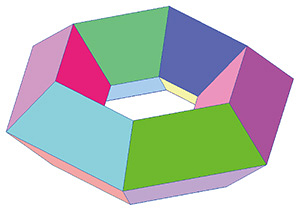
A continuous deformation means regarding a surface as a ‘soft rubber’ and transforming it without tearing. As an application of this theorem, let us do the following exercise: can we continuously deform the surface in Fig. 1(a) into the one in Fig. 1(b)? Apparently, the genus of Fig. 1(a) is 2, and that of Fig. 1(b) is 3. Thanks to the theorem, any surface obtained by a continuous deformation of Fig. 1(a) remains having genus 2, not 3. This shows that Fig. 1(a) can never be continuously deformed to Fig. 1(b).

This conclusion could be intuitively obvious since these surfaces have simple structures. However, what if a surface has a trillion holes? At least to me, it is completely non-obvious that the number of holes will not change after any continuous deformation of the surface. The point of the above theorem is that the result is mathematically proven true for any extreme examples outside our imagination.

4. How to ‘see’ the invisibles

In the previous example, we could count the number of holes by directly seeing the figures. However, we will not be able to do this for ‘invisible’ shapes, which often appear in the study of mathematics. Therefore, let us think of another method of calculating the genus of surfaces. As the above theorem says, the genus is unchanged by any continuous deformation. Therefore, we can replace the surface of a donut with a polyhedron, as in Fig. 2. We then have the following surprising theorem:

Theorem: If the genus of a polyhedron is g, then we have #(vertices) – #(edges) + #(faces) = 2–2g.

Fig. 2. Polyhedron of genus 1.

Here, #(vertices) means the number of vertices on the polyhedron, and similarly for edges and faces. Also, the alternating sum #(vertices) – #(edges) + #(faces) is called the Euler characteristic. By direct counting, we can check if the theorem is true for the surface in Fig. 2: it has 24 vertices, 48 edges, and 24 faces. And the genus is g = 1. Substituting them into the equation in the theorem, both sides have the same value 0. This works. If one has a pencil and piece of paper, it would be a fun exercise to try other examples, e.g., a hexahedron. In this case, the genus is g = 0.

In the above example, we could easily and directly count the number of holes since we could see the entire surface structure. If we live on the surface (like we live on the earth, a sphere), however, counting the number of holes would be much more difficult. Even in this situation, the above theorem ensures that we can ‘compute’ the genus by dividing the surface into a polyhedron and by counting the numbers of vertices, edges, and faces (which should be possible by moving around on the surface without seeing it from the universe).

This approach can be applied not only to surfaces but also to geometric objects (shapes) of higher dimensions. A (two-dimensional) polyhedron consists of three types of ‘parts’—vertices, edges, and faces. These are also called cells. A shape that can be continuously deformed to an n-dimensional disk is generally called an n-cell. A vertex is a zero-dimensional disk, so it is a zero-dimensional cell. Similarly, an edge is a one-dimensional cell, and a face is a two-dimensional cell (the faces of a polyhedron are angular, but they are continuously deformed to a disk). A shape constructed by combining cells is called a cell complex^*1 (a polyhedron is a two-dimensional cell complex). Just as a surface could be continuously deformed to a polyhedron, a large part of higher dimensional shapes can be deformed to cell complexes. Cell complexes contain concrete information, such as the number of cells in each dimension and how two cells are connected (or non-connected) by another cell (e.g., we can ask whether two vertices are connected by an edge). Such information reveals important properties of ‘invisible’ shapes living in higher dimensions.

5. Cohomology

The Euler characteristic depends only on the number of cells in each dimension appearing in the polyhedron and does not use the information of the relationship between the cells. By using this extra information, we can construct the cellular cohomology^*2, which drastically upgrades the Euler characteristic of a surface. The Euler characteristic assigns values to shapes, while the cellular cohomology assigns vector spaces to shapes.

Let us use the letter X to denote the shape we want to study, and let d be the dimension of X. Suppose also that X is a cell complex (by applying continuous deformation). Then there are (d + 1)-types of cells appearing on X—cells of 0, 1, 2, …, d dimensions. The cellular cohomology is given as d + 1 vector spaces^*3 corresponding to the dimensions of cells, which are usually written as

H⁰(X), H¹(X), H²(X), …, H^d(X).

Usually, we abbreviate the collection of these d + 1 vector spaces as H^＊(X) to simplify the notation. When X has dimension 2 (i.e., if X is a surface), then the cellular cohomology of X consists of three vector spaces H⁰(X), H¹(X), H²(X). Any vector space has dimension, and if X is a surface, then the Euler characteristic of X coincides with the alternating sum of the dimensions of these three vector spaces. Thus, we can regard the cellular cohomology as a generalization of the Euler characteristic.

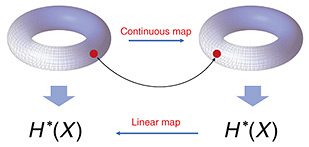
6. Functoriality of cohomology

The cellular cohomology has much richer information than the Euler characteristic. To see this, we should consider not only the shapes but also the continuous maps between them. By the cellular cohomology, a linear map H^＊(Y) → H^＊(X) is assigned to a continuous map^*4 X → Y. This property is called the functoriality of the cellular cohomology (Fig. 3). If we are given the data of ‘objects’ and ‘maps (morphisms) between objects’ satisfying suitable conditions, they are generally called a category. If we have two categories and a rule to assign objects and morphisms of one of them to those of the other, it is called a functor. Using these terminologies, we can say that the cellular cohomology is a functor from the category of CW complexes to the category of (graded) vector spaces.

Fig. 3. Functoriality of cohomology.

The functoriality of the cellular cohomology extracts much information from continuous maps. Indeed, it transforms any continuous map to a linear map, and any linear map can be represented by a matrix after fixing the basis of the vector spaces. A matrix is simply a table of numbers, which is nothing but numerical data. By applying the theory of linear algebra such as determinant, trace, and eigen values, we can obtain essential information of the matrix, hence of the continuous map we started from.

The functoriality is also useful in the study of the symmetry of shapes, which is mathematically an action of a group on a shape (e.g., rotation of a circle). If the action on a shape X is continuous, then each member of a group gives a continuous map X → X, and the functoriality of the cellular cohomology induces a linear map H^＊(X) → H^＊(X). This is nothing but a representation of the group.

7. Cohomology in arithmetic geometry

Now, let us go back to arithmetic geometry. The aim of arithmetic geometry is to study the properties of algebraic varieties, i.e., the graphs of algebraic equations. If we consider the solutions in real (or complex) numbers, then the graphs have continuous nature since the set of real or complex numbers has a continuous geometric structure. Hence, we can apply the cellular cohomology to study graphs.

However, the main target of number theory is the solutions in integers, rational numbers, etc. These numbers are non-continuous, hence, so are the graphs. It is not a good idea to apply cellular cohomology to study such non-continuous graphs since it was developed to capture the continuous nature of shapes.

To overcome this difficulty, Alexander Grothendieck, a founder of arithmetic geometry, introduced the étale cohomology as an analog of cellular cohomology in the context of arithmetic geometry. He and his collaborators proved and published the fundamental results on étale cohomology [1]. Similarly to the cellular cohomology, the étale cohomology assigns vector spaces to algebraic varieties and has a certain functoriality (we must replace ‘continuous maps’ with ‘morphisms of algebraic varieties’). The main idea of cellular cohomology is to regard a shape as a structure built with small pieces (cells) and extract global information from those pieces. The idea of étale cohomology is similar—we split algebraic varieties into small pieces (in a suitable sense) and glue them to recover the global structure—but its actual construction uses many abstract concepts such as categories, functors, and sheaves developed in the 20th century. This abstract approach is not so-called abstract nonsense. Grothendieck used these abstract concepts to upgrade the concepts from the usual geometry.

The theory of étale cohomology is abstract and complicated but very powerful and has continuously provided many applications in arithmetic geometry, including the proof of the Weil conjecture (an analog of the Riemann hypothesis) by Deligne [2] and the proof of Fermat’s last theorem by Wiles [3, 4]. It might be fair to say that arithmetic geometry cannot even exist without the theory of étale cohomology.

Modern mathematics has created many new concepts, including categories, functors, and sheaves. The extremely abstract nature of those concepts often gives the impression that mathematicians are deliberately trying to make things difficult. However, these abstract concepts were created to achieve simple goals, such as ‘to create a meaningful geometry even in a discontinuous world’. Throughout history, new mathematical concepts were often considered abstract and without substance but were widely accepted by societies afterwards. Negative numbers and complex numbers are good examples, and cohomology is becoming one of them. Cohomology has been a powerful tool for capturing structures and patterns in data, opening a new field of topological data analysis providing new applications.

8. Motive

In addition to étale cohomology, various other cohomologies have been developed for different applications. Examples include de Rham cohomology, which extracts the differential geometrical structure of algebraic varieties, and crystalline cohomology, which extracts the analytic structure in the world of numbers with positive characteristics. These are created by focusing on different aspects of algebraic varieties and are seemingly unrelated to each other at first glance. Nevertheless, these different cohomologies share common properties. Various comparison theorems also hold. In other words, in certain settings, different cohomologies can be isomorphic.

Why is there such a deep relationship between cohomologies coming from very different contexts? Is it simply a coincidence? Grothendieck’s answer was ‘no’. He conjectured that ‘behind the cohomologies of algebraic varieties, there must be a universal object unifying them’ and named this hypothetical object ‘motive’ [5].

The term motive (motif in French) originally meant the ‘driving force’ of the creation of art works, such as music or paintings. Grothendieck seems to have used this term to mean a driving force creating various cohomologies. In fact, Grothendieck developed his theory by constructing the motive theory for cohomologies of algebraic varieties under the assumption that algebraic varieties are projective^*5and smooth. His theory is now called the theory of pure motive.

9. Mixed motive

However, Grothendieck’s theory can be applied only to cohomologies for projective smooth varieties. In fact, most of the cohomologies for projective smooth varieties are generalized for smooth varieties that are not necessarily projective, and they are very important in arithmetic geometry. Thus, after Grothendieck, there were many attempts to generalize the theory of pure motive by removing the projectivity condition. The result was the theory of mixed motives, which was constructed independently by Masaki Hanamura, Marc Levine, and Vladimir Voevodsky in different formulations. Let us discuss Voevodsky’s method [6].

Roughly speaking, Voevodsky’s idea is to construct an analogue of cellular cohomology (or, more generally, singular cohomology) in the framework of algebraic geometry. As mentioned above, it is difficult to capture number-theoretic information (e.g., solutions in rational numbers) of algebraic equations by using the usual cellular cohomology. This is because the continuous deformation kills such information—whether a point on the graph is a solution in rational numbers is completely lost if the point is moved even slightly.

Voevodsky constructed the concept of continuous deformation that makes sense even in the discontinuous world of integers and rational numbers. Mathematically, the usual continuous deformation inside a space X is formalized as a continuous map from the product of X and the real number line to X. In other words, the real number line plays the role of the space of deformation parameters (i.e., time axis). However, as explained above, the real number line (which is a continuous space) cannot be used to capture number-theoretic information. Therefore, instead of the real number line, Voevodsky used the affine line, which is a convenient algebraic variety that represents a ‘one-dimensional coordinate axis’ regardless of the range in numbers under consideration. It corresponds to the real number line in the world of real numbers and to the complex plane in the world of complex numbers (the complex plane is a one-dimensional space represented by one complex variable, though it is two-dimensional from the standpoint of real numbers).

Voevodsky’s idea is very simple, but there were many technical difficulties to overcome. He successfully established his theory in a very satisfactory way. As naturally expected from the design, his theory produces an algebro-geometric analogue of cell complex (and its generalization, singular complex), which is called the mixed motive. The mixed motive has the information of various cohomologies of algebraic varieties. For example, singular cohomology, étale cohomology^*6, and de Rham cohomology can all be derived from the mixed motive. In other words, the mixed motive is the ‘seed’ of the various cohomologies. Voevodsky used his theory to prove a new comparison theorem for cohomologies, called the Milnor conjecture (and its generalization, the Bloch–Kato conjecture), for which he received the Fields Medal.

10. Towards a further generalization of motive

One of the most important and fundamental properties of the mixed motive is homotopy invariance. In the usual theory of continuous deformation, we use the real number line as the space of the deformation parameter. This automatically implies that a real number line can be continuously deformed to a single point. If we consider a continuous deformation that transfers a point x on the real number line to the point (1 – t)x at time t, the point at the initial position (1 – 0)x = x will be moved to the origin (1 – 1)x = 0 at time t = 1.

In the theory of mixed motives, the affine line is used as a replacement of the real number line. Therefore, the affine line is ‘continuously deformed’ to a single point for the same reason as above. This, in turn, means that in the theory of mixed motives, there is no distinction between the affine line and a single point. This property is called the homotopy invariance of mixed motive.

Homotopy invariance is powerful, implying various useful facts about mixed motives. However, it also imposes a fundamental restriction: the cohomology captured by the theory of mixed motive is limited to those satisfying homotopy invariance, while many cohomologies in arithmetic geometry do not satisfy homotopy invariance.

My collaborators and I have therefore constructed the theory of ‘motives with modulus’ that generalizes the theory of mixed motive by replacing homotopy invariance with a ‘weaker’ property and recasting the whole theory from scratch [7–9]. Many useful cohomologies appearing in arithmetic geometry are expected to be controlled by this new framework. Cohomologies that do not satisfy homotopy invariance, including cohomology of the structure sheaf, Hodge cohomology, cyclic cohomology, and Hodge–Witt cohomology have been proven to be controlled by the theory of motives with modulus.

11. Future perspectives

The theory of mixed motives is expected to control a wide class of cohomologies not captured by the classical motive theory. Our future aim is to control the theory of p-adic cohomologies, which has made remarkable progress. The étale cohomology referred to in this article is precisely what is often referred to as l-adic étale cohomology (l-adic cohomology for simplicity). The slogan is that l-adic cohomology captures the topological aspects of algebraic varieties, whereas p-adic cohomologies focus on the analytic aspects. Despite this difference, it is observed that there are interesting similarities and correspondences between the two. Therefore, it is naturally expected that there could be a hidden ‘motive’ behind them. An obvious problem is that p-adic cohomologies (at least part of them) are not homotopy invariant and cannot be captured using the classical motive theory. However, if p-adic cohomologies can be controlled by the theory of motives with modulus, comparing these theories on a common ground will become possible. The future success of our attempt will elucidate the unknown mechanism by which mysterious similarities between cohomologies are produced and will significantly impact the entire study of number theory.

References

[1]	M. Artin, A. Grothendieck, and J.-L. Verdier (eds.), “Théorie des Topos et Cohomologie Etale des Schémas. Séminaire de Géométrie Algébrique du Bois-Marie 1963-64 (SGA4),” Springer-Verlag, Berlin, Heidelberg, New York, 1972.
[2]	P. Deligne, “La Conjecture de Weil. I,” Publications Mathématiques de L’Institut des Hautes Études Scientifiques, Vol. 43, pp. 273–307, 1974. https://doi.org/10.1007/BF02684373
[3]	A. Wiles, “Modular Elliptic Curves and Fermat’s Last Theorem,” Annals of Mathematics, Vol. 141, No. 3, pp. 443–551, 1995.
[4]	R. Taylor and A. Wiles, “Ring-Theoretic Properties of Certain Hecke Algebras,” Annals of Mathematics, Vol. 141, No. 3, pp. 553–572, 1995.
[5]	J. Milne, “Motives — Grothendieck’s Dream,” 2012. https://www.jmilne.org/math/xnotes/MOT.pdf
[6]	V. Voevodsky, “Triangulated Categories of Motives over a Field,” Cycles, Transfers, and Motivic Homology Theories, Vol. 143, pp. 188–238, Princeton Univ. Press, 2000. https://doi.org/10.1515/9781400837120.188
[7]	B. Kahn, H. Miyazaki, S. Saito, and T. Yamazaki, “Motives with Modulus, I: Modulus Sheaves with Transfers for Non-proper Modulus Pairs,” Épijournal de Géométrie Algébrique, epiga:5979, 2021. https://doi.org/10.46298/epiga.2021.volume5.5979
[8]	B. Kahn, H. Miyazaki, S. Saito, and T. Yamazaki, “Motives with Modulus, II: Modulus Sheaves with Transfers for Proper Modulus Pairs,” Épijournal de Géométrie Algébrique, epiga: 5980, 2021. https://doi.org/10.46298/epiga.2021.volume5.5980
[9]	B. Kahn, H. Miyazaki, S. Saito, and T. Yamazaki, “Motives with Modulus, III: The Categories of Motives,” Ann. K-Theory, Vol. 7, No.1, pp. 119–178, 2022. https://doi.org/10.2140/akt.2022.7.119